# Risk Assessment Classification Taxonomy
The risk classification taxonomy comprises of four classes of risk assessments that Arup performs: Class 1, Class 2, Class 3, and Class 4. For comparison purposes, a "Class 0" is also summarized, as this is a type of risk assessment that some competitors provie.
For a given asset and hazard, the methodology for each risk assessment class follows the same generic procedure:
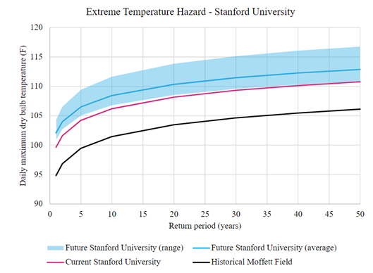
- Quantify hazard. This requires a representation of the return period and intensity of the relevant hazard. For a Class 1 risk assessment, depending on the available information, this could be as simple as characterizing the return period and intensity of a single representative event (e.g., the 500-year flood depth). For higher classes of risk assessments, it is more common to develop a hazard curve, which contains multiple likelihood / intensity pairs (e.g., the 10-year, 50-year, 100-year, 500-year, and 1,000-year flood depths) and can be plotted into a curve. See example hazard curves below.
Figure 2. Example of a set of hazard curves. This figure depicts hazard curves representing extreme temperatures near Stanford University, including a projection of “future” hazard, which is different from current hazard due to climate change impacts.
Quantify exposure. This requires a representation of the asset's characteristics. For a Class 1, this could be as simple as the identification of a generic archetype (e.g. "modern high-rise office building"). For Class 3 and 4 assessments, developing an exposure model typically includes identifying types, locations, and quantities of components within the asset (e.g. "the office building has 3 transformers on the ground floor"). The exposure model for a Class 3 or Class 4 assessment could also include information about the number of occupants in the asset, the criticality of the asset to an overall system, and/or the presence of backup utility operations.
Quantify vulnerability. This requires a representation of what level of hazard intensity will trigger a state of damage for the asset. For a Class 1 risk assessment, this could be as simple as a binary threshold at a hazard intensity level (e.g., “at 2 feet of flooding, the asset will experience significant damage”). If there is limited information about the hazard, such as only a single return period and associated hazard intensity, then the vulnerability quantification may be tied to the intensity at that single return period (e.g., “all that is known is that the 500-year flood depth is 1 foot. At this flood depth, the asset will experience minor damage”).
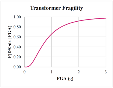
For higher classes of risk assessments, it is more common to develop fragility curves, often represented as cumulative probability distributions, which relate hazard intensities to the probabilities of incurring different damage states. For Class 1 and Class 2 risk assessments, these fragility curves are generally at the asset level (e.g., the probability that the asset experiences different damage states), but for Class 3 and 4 assessments, these fragility curves are at the component level (e.g., the probability that components within the asset experience different damage states). See example fragility curve below.
Figure 3. Example of a fragility curve. This figure depicts a fragility curve for a utility transformer under seismic shaking. Here, the x-axis represents the intensity measure for seismic shaking, which is peak ground acceleration (PGA), and the y-axis represents the probability of exceeding a specified damage state (DS).
- Quantifying consequences. This requires a representation of the consequences of the damage state(s) considered in the vulnerability analysis. The types of consequences, or “risk metrics,” may vary by client, but common risk metrics include (but are not limited to) repair cost, downtime, injuries, and fatalities. For a Class 1 risk assessment, the quantification of consequences sometimes involves assigning the consequences of the considered damage state(s) into “buckets,” such as weeks or months of downtime, or 1%-3% repair cost or 3%-10% repair cost (as a fraction of replacement value).
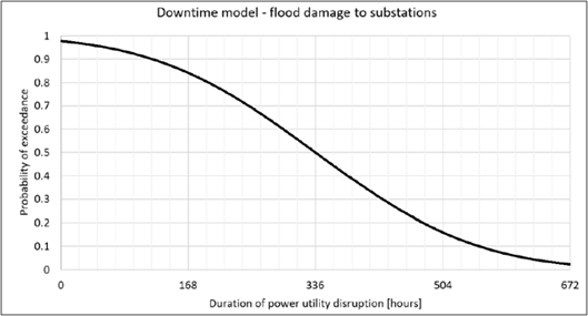
For higher classes of risk assessments, it is more common to develop consequence curves, often represented as cumulative probability distributions, which for a given damage state, express the probability of different consequence levels. See example consequence curve below.
Figure 4. Example of a consequence curve. This figure depicts a consequence curve for a damage state caused by flood damage to a utility substation. The x-axis represents the consequence level, which in this case is the duration of the associated power utility disruption. The y-axis is the probability that a given duration will be exceeded if the damage state is experienced.
There are a few critical features of the methodologies underpinning these risk assessment classes that make them cohesive and consistent with each other:
Each of the risk assessment classes could, in theory, be applied to any type of hazard, asset, or risk metric (i.e., financial loss, downtime, etc.).
Each of the risk assessment classes requires quantification of hazard, exposure, vulnerability, and consequences. Even for Class 1 assessments, which are indicated as being qualitative because the final risk ratings are descriptors (e.g., High, Medium, and Low), the choice of which risk rating to assign is underpinned by risk quantification.
None of the risk assessment classes are “conservative” in nature. That is, it is not expected that Class 3 or Class 4 assessments would systematically show lower risks than Class 1 or Class 2 assessments for the same hazard, asset, and risk metric.
The risk assessment classes are “backwards compatible,” in that the results of a higher-class assessment could be directly converted into a lower-class assessment. For example, if a Class 3 assessment is performed, providing component-level loss distributions, the results could be directly converted into the Low / Medium / High metrics typically output from a Class 1 assessment.
A detailed comparison of the different risk classes can be found in the table below:
Table 2. Details of four different classes of risk assessments that Arup performs. ^Class 0 is included for comparison, but Arup does not perform Class 0 assessments.
| Arup Risk Assessment Classes - For Property | |||||
|---|---|---|---|---|---|
| Class 0^ | Class 1 | Class 2 | Class 3 | Class 4 | |
| General description | Rapid hazard and exposure assessment | Rapid risk screening assessment | Enhanced risk screening assessment | Component level, in-depth risk modeling | Component level, physics-based vulnerability |
| Application | Pre-screening for more detailed risk assessment Awareness | Screening for more detailed risk assessment Site selection / Due diligence Awareness Reporting | Screening for Class 3 or 4 risk modeling Indications of vulnerable components Site selection / Due diligence Risk-informed decision-making Awareness Reporting | Identification of components driving risk Component-specific risk mitigation Cost-benefit analysis and insurance optimization | Identification of components driving risk Component-specific risk mitigation Cost-benefit analysis and insurance optimization Resilience-based design of new buildings |
| Recommended scale | 1,000’s of buildings | 100’s to 1,000’s of buildings | 10’s to 100’s of buildings | 10’s of buildings | |
| Accuracy / confidence | Very Low | Low | Medium | High | Very High |
| Methodology | Automated/td> | Standard desktop study OR Generic semi-quantitative (w/o engineering judgement) | Enhanced desktop study OR Site specific semi-quantitative (w/engineering judgement) | Fully probabilistic and quantitative | |
| Hazard analysis | Coarse indicators | Public maps (e.g., FEMA) Moderate-fidelity quantitative data | Moderate-fidelity quantitative data Statistical analysis relating intensity to probability May include basic site-specific adjustments (e.g., public flood maps don’t include site grading changes) | High resolution site-specific modeling Probabilistic hazard analysis Typically two-dimensional | Site-specific modeling Probabilistic hazard analysis Typically three-dimensional, physics-based Highest resolution |
| Exposure quantification | Geo-location | Basic building information based on archetype | Basic building information based on archetype supplemented with site-specific data on important building features | Normative component information supplemented with site-specific data for some important metrics | Actual component information |
| Vulnerability / exposure analysis | None | Basic asset information per archetype Estimate high-level damage potential | Archetype/Building scale loss curves with secondary modifiers | Generic component scale fragility curves supplemented with client-specific fragility curves Simplified EDP analysis supplemented with engineering calculations | 3D modeling of component response to static and dynamic loads Custom fragility curves |
| Risk Quantification | Scoring | Building-level analysis (e.g., ASTM 2027) | Building-level analysis with some component information (e.g., HAZUS, insurance catastrophe modeling) | Component-level modeling (e.g., FEMA P-58, REDi risk modeling) | |
| Typical metrics | Index scoring | Low, Medium, High | Low, Medium, High OR Best-estimate for damage, downtime, financial loss, and/or casualties | Fully-probabilistic estimates for damage, downtime, financial loss, and casualties Business interruption losses Population displacement | |
| Level of effort | ¢ “Seconds” | $ “Minutes” (with archetypes) “Hours” (without) | $$ “Hours” (with archetypes) “Days” (without) | $$$ “Days” | $$$$ “Weeks” |